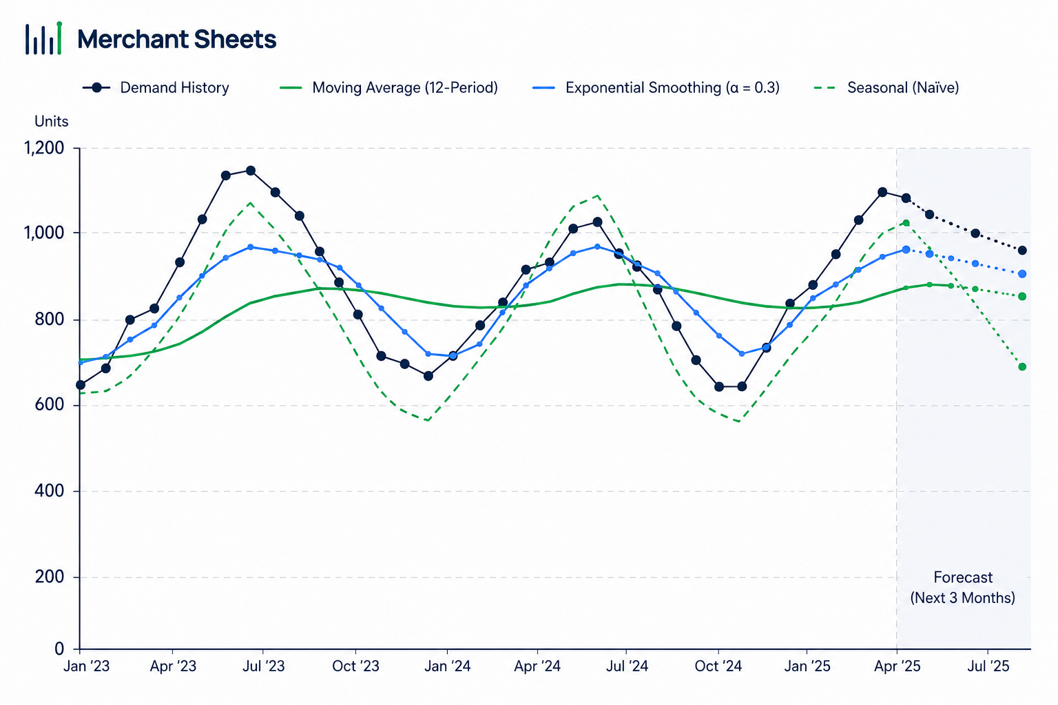
Demand Forecasting: Methods, Formulas & Common Mistakes

Demand forecasting turns your sales history into a number you can plan around: how much to buy, when to reorder, and how much cash it ties up. The methods behind it aren’t complicated, and most ecommerce catalogs run on three or four of them. What trips operators up usually isn’t the math. It’s a handful of quiet mistakes that skew the inputs before a formula ever runs.

This guide walks through the core methods, works each formula on real numbers, shows you how to pick the right one for a given product, and covers the mistakes that break a forecast.

What is demand forecasting?

Demand forecasting is the practice of estimating how many units you’ll sell in a future period, built from historical demand and any other signal you trust. It produces a plan-ready number that drives what you buy, when you reorder, and how much cash you commit to inventory. The aim is a forecast you can plan around, even if it’s never exact.

Every downstream inventory number starts here. Your forecast sets the baseline for safety stock, feeds the reorder point that tells you when to buy, and lands in the cash plan as the biggest use of working capital most brands carry. It’s the first step in a wider inventory planning framework, and a tighter forecast shows up downstream as healthier inventory turnover and less cash stranded on the shelf.

A forecast that’s off by 20% doesn’t stay a forecasting problem; it becomes a stockout, a cash crunch, or a warehouse full of product that won’t sell.

Why demand forecasting matters for an ecommerce business

Get the number too high and you sink cash into stock that sits, racks up storage, and ages toward markdowns. Get it too low and you stock out, lose the sale, and often lose the customer to a competitor who had it on the shelf. The forecast is the first domino, and everything from your safety stock buffer to your weekly cash flow depends on it landing close.

That’s why forecasting is worth doing well even when it’s rough. A directional forecast you revisit every month beats a precise one you build once and forget, because demand moves and the plan has to move with it. The same number becomes the base case you flex in scenario planning and the trigger you time your restocks around.

Demand vs sales: the distinction that decides everything

Here’s the piece most forecasts get wrong before any math happens. Your sales history is not your demand history. Sales are what you managed to fulfill; demand is what customers wanted. The two only match when you never stocked out, never ran a promo, and never took a return, which is to say almost never.

Feed raw sales into a forecast and you teach it your past constraints. A month you sold out early looks like soft demand, so the model tells you to buy less, and you stock out again. Clean the history first:

• Stockouts: When an item sold out mid-period, recorded sales stop at the shelf, not at true demand. Flag those periods and estimate what would have sold, or leave them out of the baseline.
• Returns: Returned units inflate gross sales. Forecast on net units so you’re not planning to restock things that came back.
• Promotions: A promo spike is borrowed demand that inflates your baseline. Separate promoted periods so a one-week sale doesn’t reset your run-rate.

Qualitative or quantitative: which should you use?

Forecasting methods fall into two families. Quantitative methods project from clean numerical history and are the workhorses for any product with a sales record. Qualitative methods lean on human judgment when the numbers don’t exist yet, like a new product launch or a market shift the data hasn’t caught. The strongest forecasts blend both: a quantitative baseline, adjusted for what your team knows that the data can’t.

This guide focuses on the quantitative formulas most catalogs run on, since that’s where the repeatable math lives.

When each family fits:

Family	Best when	Methods	Trade-off
Quantitative	You have clean sales history	Moving average, exponential smoothing, seasonal index, regression	Objective and repeatable, but blind to anything not in the data
Qualitative	New product, no usable history, or a big market shift	Expert judgment, sales-team input, customer surveys	Fast and context-aware, but subjective and hard to turn into a unit number

Demand forecasting formulas, worked

We’ll run one SKU through each method so the outputs compare directly. Keep everything in units and hold the grain steady, so months stay months and you’re never mixing weekly and monthly numbers in the same model. Here are six months of clean unit demand for the example SKU:

Table: monthly unit demand for one SKU

Month	Jan	Feb	Mar	Apr	May	Jun
Units	120	135	150	140	160	175

Simple moving average

A simple moving average (SMA) forecasts the next period as the plain average of the last n periods. It smooths out noise and works best for demand that’s stable with no strong trend or season.

Simple moving average = (sum of the last n periods) ÷ n

Using a three-month window, the forecast for July is the average of April, May, and June: (140 + 160 + 175) ÷ 3 = 158 units. It’s quick and hard to argue with, but it lags a real trend. Because demand here is rising, the average of the last three months sits below the latest month, so an SMA will chase a climbing trend from behind. The choice of window is a judgment call too: a shorter window reacts faster, a longer one smooths harder.

Weighted moving average

A weighted moving average (WMA) is the same idea with the recent periods turned up. You assign larger weights to the newest months so the forecast leans toward where demand is heading, not where it’s been.

Weighted moving average = Σ(period × weight) ÷ Σ(weights)

Weight the last three months 3 for June, 2 for May, 1 for April: (175×3 + 160×2 + 140×1) ÷ (3 + 2 + 1) = 985 ÷ 6 = 164 units. That’s six units above the simple average, because the WMA gives the rising recent months more say. The catch is that the weights are yours to pick, so two people can build two different forecasts from the same data.

Exponential smoothing

Exponential smoothing carries the same intuition further. Each new forecast is a blend of the latest actual and the previous forecast, controlled by a smoothing factor, alpha (α), between 0 and 1. A high alpha reacts fast to recent change; a low alpha smooths hard and moves slowly.

Next forecast = α × (latest actual) + (1 − α) × (last forecast)

Seed the first forecast with January’s actual (120) and run it forward with α = 0.3:

Table: exponential smoothing at α = 0.3

Month	Actual	Forecast (α = 0.3)
Feb	135	120
Mar	150	124
Apr	140	132
May	160	135
Jun	175	142
Jul	n/a	152

The July forecast of 152 units sits below both moving averages because a low alpha is still catching up to the climb. Raise alpha and it tracks the trend more closely at the cost of reacting to every blip. Exponential smoothing shines when demand is drifting up or down and the most recent months carry the most signal.

Seasonal forecast: baseline times a seasonality index

Most catalogs have a season, and none of the methods above can see it, because a trailing average has no idea December isn’t March. A seasonal forecast fixes that by splitting demand into a baseline run-rate and a set of seasonality indices, one per period, that say how far above or below average that period usually runs.

Seasonality index = period average ÷ overall average    →    Forecast = deseasonalized baseline × the period’s index

You need about two years of history to read a season cleanly. Take this quarterly demand for a SKU with a Q4 holiday peak:

Table: two years of quarterly demand and the resulting seasonality index

Quarter	Year 1	Year 2	2-yr average	Seasonality index
Q1	800	880	840	0.80
Q2	900	1,000	950	0.90
Q3	850	950	900	0.86
Q4	1,450	1,570	1,510	1.44

The grand average is 1,050 units per quarter, so each index is that quarter’s two-year average divided by 1,050. Q4 runs 44% above a normal quarter; Q1 runs 20% below.

To forecast Year 3, start from the deseasonalized baseline, the trailing-year run-rate of 4,400 ÷ 4 = 1,100 units per quarter, then re-apply each index: Q1 = 1,100 × 0.80 = 880, Q2 = 990, Q3 = 946, and Q4 = 1,100 × 1.44 = 1,584 units.

Forecast the deseasonalized run-rate first, then re-apply the seasonality index. Projecting raw seasonal months straight forward bakes last year’s spikes into next year’s plan.

Linear trend

When demand climbs or falls in a fairly straight line, a linear trend fits a best-fit line through the history and extends it. In y = a + b × (period), b is the slope, the average change per period, and a is the starting level.

It’s the idea behind the FORECAST.LINEAR function, and it pairs well with the seasonal method: fit the trend to the deseasonalized baseline, then layer the indices back on.

Watch the horizon, though, since a straight line drawn too far out assumes a growth rate that rarely holds.

These are the formulas at the concept level. To build them cell by cell with AVERAGE, SUMPRODUCT, FORECAST.ETS, and FORECAST.LINEAR, follow the step-by-step version and forecast demand in Excel.

How do you choose a forecasting method?

Match the method to the demand pattern, then confirm the choice with a quick backtest. Flat, stable demand wants a moving average; a steady climb or decline wants exponential smoothing or a linear trend; a seasonal catalog wants a seasonal index; and a product with no usable history falls back on qualitative judgment until it builds a record.

Table: which method fits which demand pattern

Method	Best for (demand pattern)	Formula	Main watch-out
Simple moving average	Stable, non-seasonal demand	(sum of last n periods) ÷ n	Lags a real trend; the window is a judgment call
Weighted moving average	Stable demand, recent periods matter more	Σ(period × weight) ÷ Σ(weights)	Weights are subjective
Exponential smoothing	Demand drifting up or down	α × actual + (1 − α) × last forecast	Choosing alpha; still lags sharp turns
Seasonal index	Seasonal catalogs (most of them)	baseline × seasonality index	Needs ~2 years; you must deseasonalize first
Linear trend	Steady straight-line growth or decline	a + b × period (best-fit line)	Breaks when growth isn’t linear; don’t project too far
Qualitative	New products, no usable history	Structured expert or sales input	Bias; hard to translate to a unit number

Backtesting settles any ties. Hold out the last three to six periods, forecast them with each candidate method as if you didn’t know the answer, and compare the results to what happened. The method with the lowest error wins, and you re-run the test as the SKU builds more history.

How do you know if your forecast is any good?

Score it, don’t eyeball it. Two numbers do the job: mean absolute percentage error (MAPE) tells you how far off you are on average, and bias tells you which direction you lean. A forecast can have a respectable MAPE and still run consistently low, which quietly starves your reorders, so watch both.

MAPE = average of |actual − forecast| ÷ actual, across periods    ·    Bias = average of (forecast − actual)

If you forecast 158 and demand comes in at 170, the absolute error is 12 and the percentage error is 12 ÷ 170 = 7%. Average that across periods for MAPE. A positive bias means you’re forecasting high and building excess stock; a negative bias means you’re forecasting low and courting stockouts.

What counts as good depends on the product: steady sellers can hit single-digit MAPE, while spiky or low-volume SKUs run far higher, and forecasts at the category level are always tighter than single-SKU ones because the errors cancel out.

When error runs high, re-pick the method rather than trusting the number. To build these checks in a spreadsheet, work through how to measure your forecast error.

Common demand forecasting mistakes

Most broken forecasts fail the same few ways, and almost none of them are about the formula. Chasing a perfect number burns the most time, when a plan-ready one would do; the rest quietly distort the inputs before the math runs.

Table: the mistakes that break a forecast, and the fix for each

Mistake	Why it breaks the forecast	The fix
Forecasting sales, not demand	Stockout periods cap recorded sales below true demand and drag the baseline down	Flag stockouts and forecast on demand, filling or excluding those periods
Forecasting revenue, not units	A price change moves the dollars without any change in real demand	Forecast in units, then convert to dollars afterward
Projecting raw seasonal months	Last year’s spikes get baked straight into next year’s plan	Deseasonalize to a baseline first, then re-apply the seasonality index
One method for the whole catalog	A flat SKU and a seasonal SKU need different math	Match the method to each product’s pattern
Ignoring lead time	A forecast that stops at next month can’t tell you what to order today	Forecast far enough out to cover your supplier lead time and reorder cycle
Never measuring accuracy	A method you don’t score never improves	Track MAPE and bias every cycle and re-pick when error runs high
Forecasting too granular on thin data	Weekly, per-SKU forecasts on six weeks of history are mostly noise	Forecast at a grain your data supports, or aggregate up until it’s stable

Put your forecast to work

Running these methods by hand is fine for one SKU. Across a live catalog, with different demand patterns per product and a season to deseasonalize, the spreadsheet work adds up fast.

The Merchant Sheets Inventory Forecasting template does the seasonal method for every SKU: it deseasonalizes each item’s trailing twelve months, projects the next twelve with a seasonality index, and turns the forecast into a safety stock level, a reorder point, and a purchase-order date and quantity.

It’s the same demand forecasting workflow in this guide, built to run on your whole catalog at once.

Frequently asked questions